Machine Learning

Workshop 10

Titanic

In this workshop, you’ll get to experiment with the Titanic dataset to learn the basic principles of machine learning.

• survival: Survival 0 = No, 1 = Yes
• pclass: Ticket class 1 = 1st, 2 = 2nd, 3 = 3rd
• sex: Sex
• Age: Age in years
  
• sibsp: # of siblings / spouses aboard the Titanic
  
• parch: # of parents / children aboard the Titanic
  
• ticket: Ticket number
  
• fare: Passenger fare
  
• cabin: Cabin number
  
• embarked: Port of Embarkation C = Cherbourg, Q = Queenstown, S = Southampton

import pandas as pd
from sklearn.model_selection import train_test_split
from sklearn.ensemble import RandomForestClassifier
from sklearn.metrics import accuracy_score
import numpy as np
# Load the dataset
df = pd.read_csv('https://storage.googleapis.com/qm2/Titanic-Dataset.csv')
df.head()

	PassengerId	Survived	Pclass	Name	Sex	Age	SibSp	Parch	Ticket	Fare	Cabin	Embarked
0	1	0	3	Braund, Mr. Owen Harris	male	22.0	1	0	A/5 21171	7.2500	NaN	S
1	2	1	1	Cumings, Mrs. John Bradley (Florence Briggs Th...	female	38.0	1	0	PC 17599	71.2833	C85	C
2	3	1	3	Heikkinen, Miss. Laina	female	26.0	0	0	STON/O2. 3101282	7.9250	NaN	S
3	4	1	1	Futrelle, Mrs. Jacques Heath (Lily May Peel)	female	35.0	1	0	113803	53.1000	C123	S
4	5	0	3	Allen, Mr. William Henry	male	35.0	0	0	373450	8.0500	NaN	S

df[['Survived','Age', 'Pclass','Sex_int','Embarked','SibSp','Parch','Fare']].describe().round(2)

	Survived	Age	Pclass	Sex_int	SibSp	Parch	Fare
count	891.00	714.00	891.00	891.00	891.00	891.00	891.00
mean	0.38	29.70	2.31	0.35	0.52	0.38	32.20
std	0.49	14.53	0.84	0.48	1.10	0.81	49.69
min	0.00	0.42	1.00	0.00	0.00	0.00	0.00
25%	0.00	20.12	2.00	0.00	0.00	0.00	7.91
50%	0.00	28.00	3.00	0.00	0.00	0.00	14.45
75%	1.00	38.00	3.00	1.00	1.00	0.00	31.00
max	1.00	80.00	3.00	1.00	8.00	6.00	512.33

from sklearn.metrics import confusion_matrix, precision_score
import seaborn as sns
import matplotlib.pyplot as plt

df['Sex_int']=np.where(df['Sex']=="male", 0,1)
df['Embarked_int']=np.where(df['Embarked']=="S", 0,np.where(df['Embarked']=="C", 1,2))
variables=['Age', 'Pclass','Sex_int','Embarked_int','SibSp','Parch','Fare']
X = df[variables]
y = df['Survived']

# Split the dataset into training and testing sets
X_train, X_test, y_train, y_test = train_test_split(X, y, test_size=0.2, random_state=42)

# Initialize the RandomForestClassifier
rf = RandomForestClassifier(n_estimators=100, random_state=42)

# Train the model
rf.fit(X_train, y_train)

# Make predictions
y_pred = rf.predict(X_test)

true_positive = sum((y_test == 1) & (y_pred == 1))
false_positive = sum((y_test == 0) & (y_pred == 1))
true_negative = sum((y_test == 0) & (y_pred == 0))
false_negative = sum((y_test == 1) & (y_pred == 0))

# Evaluate the model
accuracy = (true_positive + true_negative) / (true_positive + false_positive + true_negative + false_negative)
precision = true_positive / (true_positive + false_positive)
recall = true_positive / (true_positive + false_negative)
f1_score = 2 * precision * recall / (precision + recall)

print(f'Accuracy: {int(accuracy*100)}')
print(f'Precision: {int(precision*100)}')
print(f'Recall: {int(recall*100)}')
print(f'F1 Score: {int(f1_score*100)}')

cm = confusion_matrix(y_test, y_pred)
#flip so tp are top left and tn are bottom right
sns.heatmap(cm, annot=True, cmap='viridis', cbar=False,square=True)
plt.xlabel('Predicted')
plt.ylabel('Labels')
plt.title(f'Confusion Matrix \nVariables: {variables}')
#change labels from 0 and 1 to 'Not Survived' and 'Survived'
plt.xticks([0.5, 1.5], ['Not Survived', 'Survived'])
plt.yticks([0.5, 1.5], ['Not Survived', 'Survived'])
plt.show()

Accuracy: 82
Precision: 80
Recall: 77
F1 Score: 78

#feature importance plot 
importances = rf.feature_importances_
indices = np.argsort(importances)[::-1]
plt.figure(figsize=(10, 5))
plt.title("Feature importances")
plt.bar(range(X_train.shape[1]), importances[indices], align="center")
plt.xticks(range(X_train.shape[1]), np.array(variables)[indices], rotation=90)
plt.xlim([-1, X_train.shape[1]])
plt.show()

Feature Engineering Exercise

we’ve gotten pretty good results using the existing features in the dataset. But we can create new features using the existing ones, and thay may help us improve accuracy.

The “Name” variabel contains the names of the passengers, including their titles:

df['Name'].head()

0                              Braund, Mr. Owen Harris
1    Cumings, Mrs. John Bradley (Florence Briggs Th...
2                               Heikkinen, Miss. Laina
3         Futrelle, Mrs. Jacques Heath (Lily May Peel)
4                             Allen, Mr. William Henry
Name: Name, dtype: object

From the names, we can identify Doctors, military officers, married and unmarried women, reverends, and more. Use natural language processing to create a new column with a value of 0 or 1 if an individual pertains to any of these classes. Add these new features to your model and see if they help us more accurately predict survival.

Optional: visuialize the random forest

from sklearn.tree import export_graphviz
import pydotplus
from IPython.display import Image

estimator = rf.estimators_[0]

# Export the tree to a dot file
dot_data = export_graphviz(estimator, out_file=None, 
                           feature_names=X.columns,  
                           class_names=['Not Survived', 'Survived'],  
                           filled=True, rounded=True,  proportion=True,
                           special_characters=True)  

# Use pydotplus to create a graph from the dot data
graph = pydotplus.graph_from_dot_data(dot_data)  

# Display the tree
Image(graph.create_png())

Deep Learning

The following goes above and beyond what we’ve learned in this class, but offers a window into the sorts of things you would learn if you chose to continue down the path of quantitative analysis. We will:

1. Load a prebuilt dataset.
2. Build a neural network machine learning model that classifies images.
3. Train this neural network.
4. Evaluate the accuracy of the model.

Set up TensorFlow

Import TensorFlow into your program to get started:

import numpy as np
import tensorflow as tf
import matplotlib.pyplot as plt

#print("TensorFlow version:", tf.__version__)

If you are following along in your own development environment, rather than Colab, see the install guide for setting up TensorFlow for development.

Note: Make sure you have upgraded to the latest pip to install the TensorFlow 2 package if you are using your own development environment. See the install guide for details.

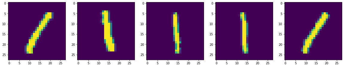
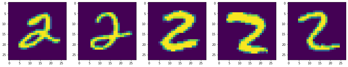
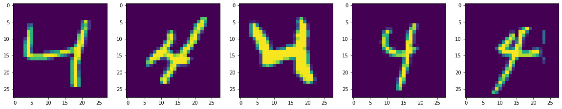
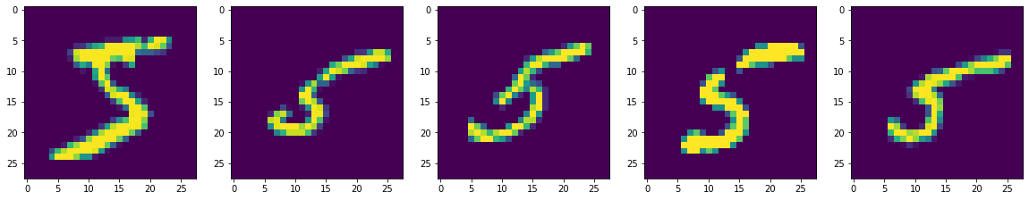
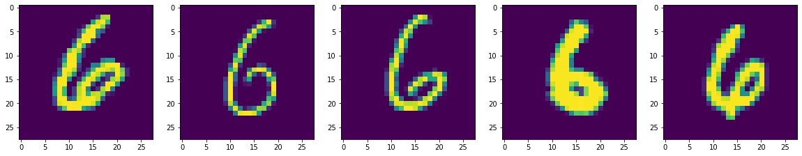
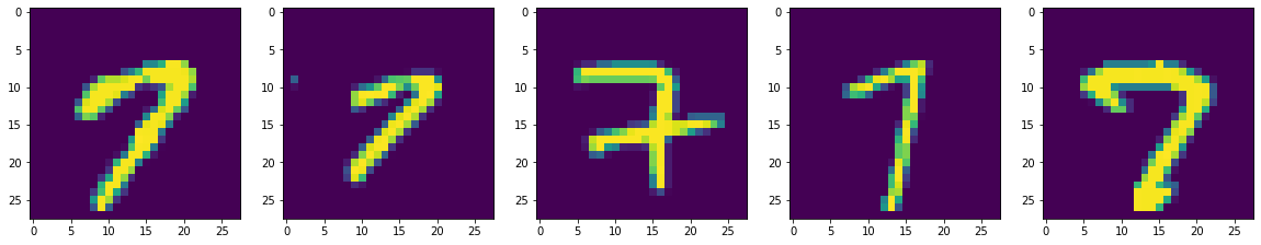
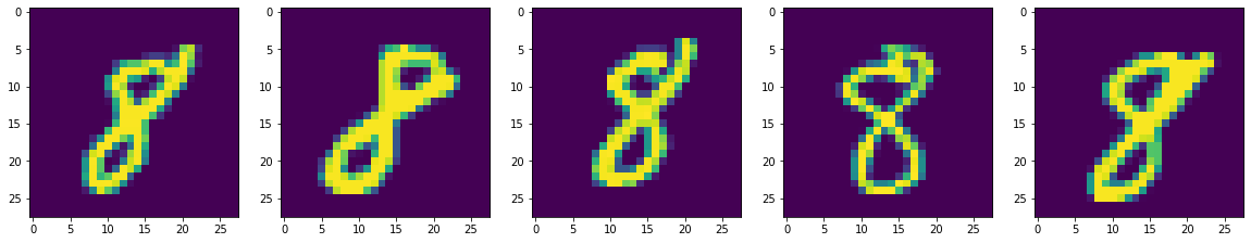
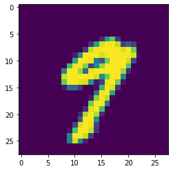
Load a dataset

Load and prepare the MNIST dataset. Convert the sample data from integers to floating-point numbers:

mnist = tf.keras.datasets.mnist

(x_train, y_train), (x_test, y_test) = mnist.load_data()
x_train, x_test = x_train / 255.0, x_test / 255.0

Downloading data from https://storage.googleapis.com/tensorflow/tf-keras-datasets/mnist.npz
11493376/11490434 [==============================] - 0s 0us/step
11501568/11490434 [==============================] - 0s 0us/step

def plot_num(number):

  item_index = np.where(y_train[:1000]==number)
  subset=x_train[item_index]
  
  egs=5
  fig, axs = plt.subplots(1,egs, figsize=(20,10))

  for i in range(0,egs):
    axs[i].imshow(subset[i])


for x in range(0,10):
  plot_num(x)

Build a machine learning model

Build a tf.keras.Sequential model by stacking layers.

model = tf.keras.models.Sequential([
  tf.keras.layers.Flatten(input_shape=(28, 28)),
  tf.keras.layers.Dense(128, activation='relu'),
  tf.keras.layers.Dropout(0.2),
  tf.keras.layers.Dense(10)
])

For each example, the model returns a vector of logits or log-odds scores, one for each class.

predictions = model(x_train[:1]).numpy()
predictions

array([[ 0.33447966,  0.35151538, -0.35632688, -0.2735348 ,  0.8568236 ,
        -0.8503612 , -0.34408805, -0.40424255,  0.4791569 , -0.00873779]],
      dtype=float32)

The tf.nn.softmax function converts these logits to probabilities for each class:

tf.nn.softmax(predictions).numpy()

array([[0.12650587, 0.12867945, 0.06340117, 0.0688737 , 0.21328573,
        0.03868484, 0.06418189, 0.06043489, 0.1461986 , 0.08975388]],
      dtype=float32)

Note: It is possible to bake the tf.nn.softmax function into the activation function for the last layer of the network. While this can make the model output more directly interpretable, this approach is discouraged as it’s impossible to provide an exact and numerically stable loss calculation for all models when using a softmax output.

Define a loss function for training using losses.SparseCategoricalCrossentropy, which takes a vector of logits and a True index and returns a scalar loss for each example.

loss_fn = tf.keras.losses.SparseCategoricalCrossentropy(from_logits=True)

This loss is equal to the negative log probability of the true class: The loss is zero if the model is sure of the correct class.

This untrained model gives probabilities close to random (1/10 for each class), so the initial loss should be close to -tf.math.log(1/10) ~= 2.3.

loss_fn(y_train[:1], predictions).numpy()

3.2523074

Before you start training, configure and compile the model using Keras Model.compile. Set the optimizer class to adam, set the loss to the loss_fn function you defined earlier, and specify a metric to be evaluated for the model by setting the metrics parameter to accuracy.

model.compile(optimizer='adam',
              loss=loss_fn,
              metrics=['accuracy'])

Train and evaluate your model

Use the Model.fit method to adjust your model parameters and minimize the loss:

model.fit(x_train, y_train, epochs=10)

Epoch 1/10
1875/1875 [==============================] - 6s 3ms/step - loss: 0.2955 - accuracy: 0.9139
Epoch 2/10
1875/1875 [==============================] - 5s 3ms/step - loss: 0.1416 - accuracy: 0.9578
Epoch 3/10
1875/1875 [==============================] - 5s 3ms/step - loss: 0.1072 - accuracy: 0.9676
Epoch 4/10
1875/1875 [==============================] - 5s 3ms/step - loss: 0.0874 - accuracy: 0.9727
Epoch 5/10
1875/1875 [==============================] - 5s 3ms/step - loss: 0.0734 - accuracy: 0.9772
Epoch 6/10
1875/1875 [==============================] - 5s 3ms/step - loss: 0.0632 - accuracy: 0.9792
Epoch 7/10
1875/1875 [==============================] - 5s 3ms/step - loss: 0.0575 - accuracy: 0.9808
Epoch 8/10
1875/1875 [==============================] - 5s 3ms/step - loss: 0.0526 - accuracy: 0.9825
Epoch 9/10
1875/1875 [==============================] - 5s 3ms/step - loss: 0.0460 - accuracy: 0.9853
Epoch 10/10
1875/1875 [==============================] - 5s 3ms/step - loss: 0.0437 - accuracy: 0.9858

<keras.callbacks.History at 0x7fe943384b10>

The Model.evaluate method checks the models performance, usually on a “Validation-set” or “Test-set”.

model.evaluate(x_test,  y_test, verbose=2)

313/313 - 1s - loss: 0.0715 - accuracy: 0.9785 - 529ms/epoch - 2ms/step

[0.07152838259935379, 0.9785000085830688]

The image classifier is now trained to ~98% accuracy on this dataset. To learn more, read the TensorFlow tutorials.

If you want your model to return a probability, you can wrap the trained model, and attach the softmax to it:

probability_model = tf.keras.Sequential([
  model,
  tf.keras.layers.Softmax()
])

#probability_model(x_test[:1])
predictions=probability_model.predict(x_test)

index=20

print(np.argmax(predictions[index]))
plt.imshow(x_test[index])

9

<matplotlib.image.AxesImage at 0x7fe9409c1ad0>

Conclusion

Congratulations! You have trained a machine learning model using a prebuilt dataset using the Keras API.

For more examples of using Keras, check out the tutorials. To learn more about building models with Keras, read the guides. If you want learn more about loading and preparing data, see the tutorials on image data loading or CSV data loading.